The first of a series of tutorial posts on Bayesian analyses. In this post I focus on using brms to run an intercept-only regression model.
Published
February 1, 2023
This post is the first of a series of tutorial posts on Bayesian statistics. I’m not an expert on this topic, so this tutorial is partly, if not mostly, a way for me to figure it out myself.
The goal will be to go through each step of the data analysis process and make things as intuitive and clear as possible. I’ll use the brms package to run the models and I will rely heavily on the book Statistical Rethinking by Richard McElreath.
The basic idea behind Bayesian statistics is that we start off with prior beliefs about the parameters in the model and then update those parameter beliefs using data. That means that for all models you need to figure out what your beliefs are before running any analyses. This is very different from frequentist statistics and probably the most off-putting part of running Bayesian analyses. However, my goal is to make this relatively easy by focusing on visualizing priors and how they change as a function of the Bayesian process. I’ll also try to come up with some methods to simplify the construction of priors, with the goal to have them be reasonable and non-controversial.
In some cases I might not even use a prior I personally believe in. Instead I’ll use a prior that represents a particular position or skepticism so that the results of the analysis can be used to change the mind of the skeptic, rather than me changing whatever I happen to believe.
With this in mind, let’s begin.
Setup
In the code chunk below I show some setup code to get started, starting with the packages. After loading the packages I set the default ggplot2 theme and some colors. Finally, I set several brms specific options to speed up the functions and automatically re-run models if a model has changed. If a model has not changed, the results will be read from a file instead of re-running the model.
The data I’ll use is the same data Richard McElreath uses in Chapter 4 of his amazing book Statistical Rethinking. The data consists of partial census data of the !Kung San, compiled from interviews conducted by Nancy Howell in the late 1960s. Just like in the book, I will focus only on people 18 years or older.
Code
data <-read_csv("Howell1.csv")data <-filter(data, age >=18)head(data)
Partial census data for the Dobe area !Kung San compiled by Nancy Howell in the late 1960s.
height
weight
age
male
151.765
47.82561
63
1
139.700
36.48581
63
0
136.525
31.86484
65
0
156.845
53.04191
41
1
145.415
41.27687
51
0
163.830
62.99259
35
1
An intercept-only model
Let’s focus the first question on the heights in the data. What are the heights of the Dobe area !Kung San?
The way to address this question is by constructing a model in which heights are regressed on only the intercept, i.e., an intercept-only model. You may be familiar with the R formula for this type of model: height ~ 1.
With this formula and the data we can use brms to figure out which priors we need to set by running the get_prior() function. This is probably the easiest way to figure which priors you need when you’re just starting out using brms.
Code
get_prior(height ~1, data = data)
prior
class
coef
group
resp
dpar
nlpar
lb
ub
source
student_t(3, 154.3, 8.5)
Intercept
default
student_t(3, 0, 8.5)
sigma
0
default
The output shows us that we need to set two priors, one for the Intercept and one for sigma. brms already determined a default prior for each parameter (they are required for a Bayesian analysis), so we could immediately run an analysis if we want to but it is recommended to construct your own priors because you can often do better than the default priors.
Also, using the get_prior() function is not the best way to think about which priors we need. Using the function will give us the answer, but it doesn’t really improve our understanding of why these two priors are needed. In this case I also omitted an important specification of the heights, which is that they are normally distributed (the default in get_prior()). So let’s instead write down the model in a different way, which explicitly specifies how we think the heights are distributed and which parameters we need to set priors on. If we think the heights are normally distributed, we define our model like this:
\[heights_i ∼ Normal(\mu, \sigma)\]
We explicitly note that the individual heights come from a normal distribution, which is determined by the parameters \(\mu\) and \(\sigma\). This then also immediately tells us that we need to set two priors, one on \(\mu\) and one on \(\sigma\).
In our intercept-only model, the \(\mu\) parameter refers to our intercept and the \(\sigma\) parameter refers to, well, sigma. Sigma is not often discussed in the literature I’m familiar with, but we’ll figure it out below. In fact, let’s discuss each of these parameters in turn and figure out what kind of prior makes sense.
The intercept (\(\mu\)) prior
The prior for the intercept refers to, in this case, the average height of the !Kung San.
brms has set the default intercept prior as a Student t-distribution with 3 degrees of freedom, a mean of 154.3 and a standard deviation of 8.5. That means brms starts off with a ‘belief’ that the average of the heights is 154.3, but with quite some uncertainty reflected in the standard deviation of 8.5 and the fact that the distribution is a Student t-distribution. A Student t-distribution has thicker tails compared to a normal distribution, meaning that numbers in the tails of the distribution are more likely compared to a normal distribution, at least when the degrees of freedom are low. At higher degrees of freedom, the t-distribution becomes more and more like the normal distribution. So, the thicker tails of the t-distributions means smaller and taller average heights are relatively more plausible.
But this is the default prior. brms determines this prior by peeking at the data to create a weak prior that is easily updated by the data. We can do a bit better than the default prior, though.
What do I believe the average height to be? As a Dutch person, I might think that the average height is around 175 centimeters. This is probably too tall to use as an average for the !Kung San because we’re known for being quite tall. So I think the average should be lower than 175, perhaps 170. I am not very sure, though. After all, I am far from an expert on people’s heights; I am only using my layman knowledge here. An average of 165 seems possible to me too. So let’s describe my belief in the form of a distribution in which multiple averages are possible, to varying extents. We could use a Student t-distribution with small degrees of freedom if we want to allow for the possibility of being very wrong (remember, it has thicker tails, so it assigns more probability to a wider range of average heights). We’re not super uncertain about people’s heights, though, so let’s use a normal distribution.
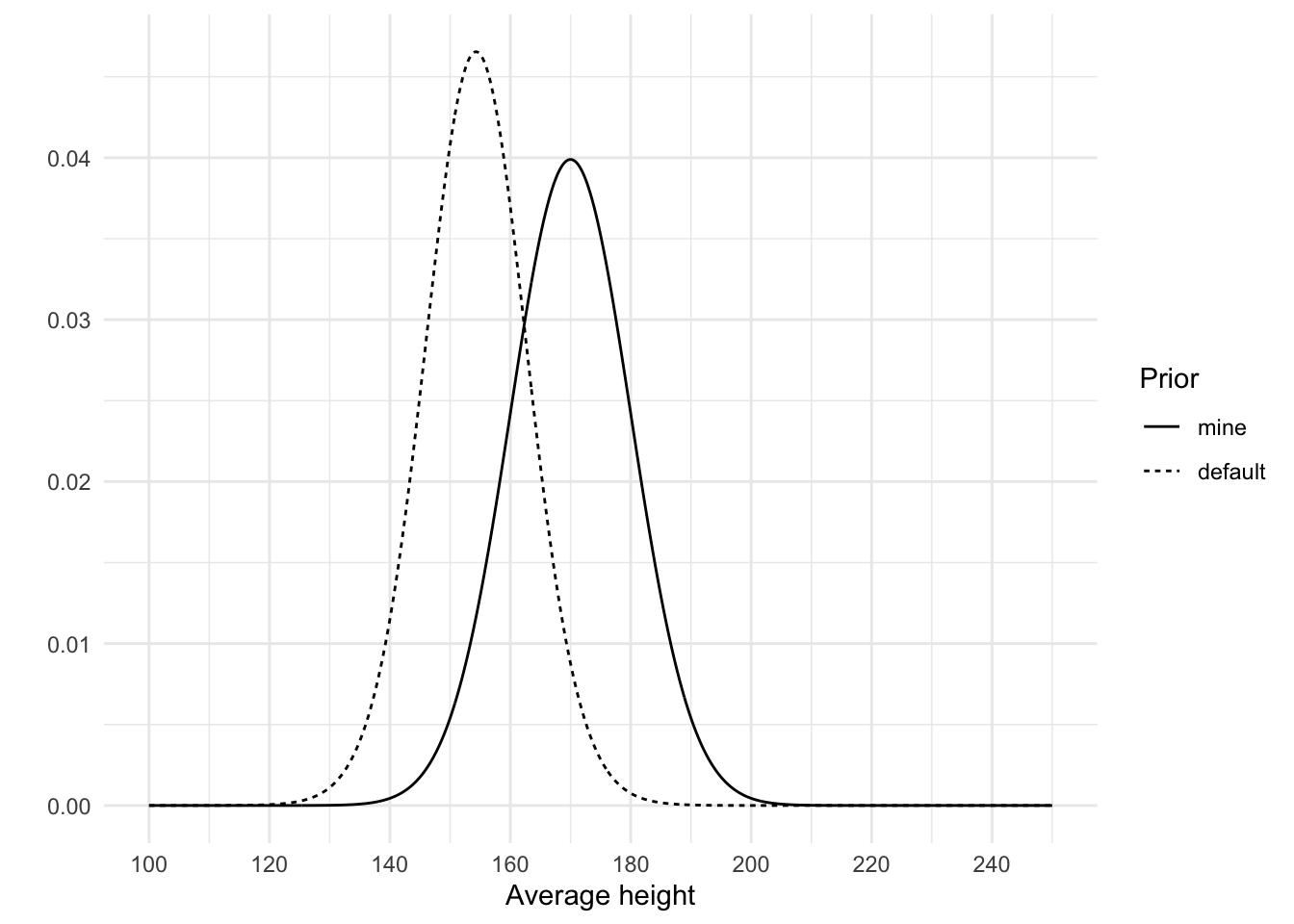
As we saw in defining our height model, a normal distribution requires that we set two parameters: the \(\mu\) and the \(\sigma\). The \(\mu\) we already covered (i.e., 170), so that leaves \(\sigma\). Let’s set this to 10 and see what happens by visualizing this prior. Below I plot both the default brms prior and our own with \(\mu\) = 170 and \(\sigma\) = 10.
Code
height_prior_intercept <-tibble(height_mean =seq(from =100, to =250, by =0.1),mine =dnorm(height_mean, mean =170, sd =10),default =dstudent_t(height_mean, df =30, mu =154.3, sigma =8.5))height_prior_intercept <-pivot_longer( height_prior_intercept,cols =-height_mean,names_to ="prior")ggplot( height_prior_intercept,aes(x = height_mean, y = value, linetype =fct_rev(prior))) +geom_line() +labs(x ="Average height", y ="", linetype ="Prior") +scale_x_continuous(breaks =seq(100, 250, 20))
Two priors for \(\mu\)
My prior indicates that I believe the average height to be higher than the default prior. In terms of the standard deviation, we both seem to be about equally uncertain about this average. Looking at this graph I think this prior of mine is not very plausible. Apparently I assign quite a chunk of plausibility to an average of 180 cm, or even 190 cm, which is very unlikely. An average of 160 cm is more plausible to me than an average of 180, so I should probably lower the mu, or use more of a skewed distribution. This is one of the benefits of visualizing the prior, it can make you think again about your prior so that you may improve on it. Based on the graph, I will change the mean of my prior to 160. I can probably also lower the standard deviation, but I’ll leave it at 10 to show how easily the data will update this prior.
The sigma (\(\sigma\)) prior
What about the sigma prior? What even is sigma? Sigma is the estimated standard deviation of the errors or, in other words, the standard deviation of the residuals of the model. In the simple case of an intercept-only model, this is identical to the standard deviation of the outcome (heights, in this case).
I think setting the standard deviation of the distribution of heights (not the mean of the heights) is quite difficult. There are parts that are easy, such as the fact that the standard deviation has to be 0 or larger (it can’t be negative), but exactly how large it should be, I don’t know.
I do know it is unlikely to be close to 0, and unlikely to be very large. That’s because I know people’s heights do vary, so I know the sigma can’t be 0. I also know it’s not super large because we don’t see people who are taller than 2 meters very often. This means the peak of our prior should be somewhere above 0, with a tail to allow higher values but not too high. We can use a normal distribution for this with a mean above 0 and a particular standard deviation, and ignore everything that’s smaller than 0 (brms automatically ignores negative values for \(\sigma\)).
As I mentioned before, there is a downside of using a normal distribution, though. Normal distributions have long tails, but there is actually very little density in those tails. If we are quite uncertain about our belief about sigma, we should use a t-distribution, or perhaps even a cauchy distribution (actually, the cauchy distribution is a special case of the t-distribution; they are equivalent if the degree of freedom is 1). The lower the degrees of freedom, the more probability we assign to higher and lower values.
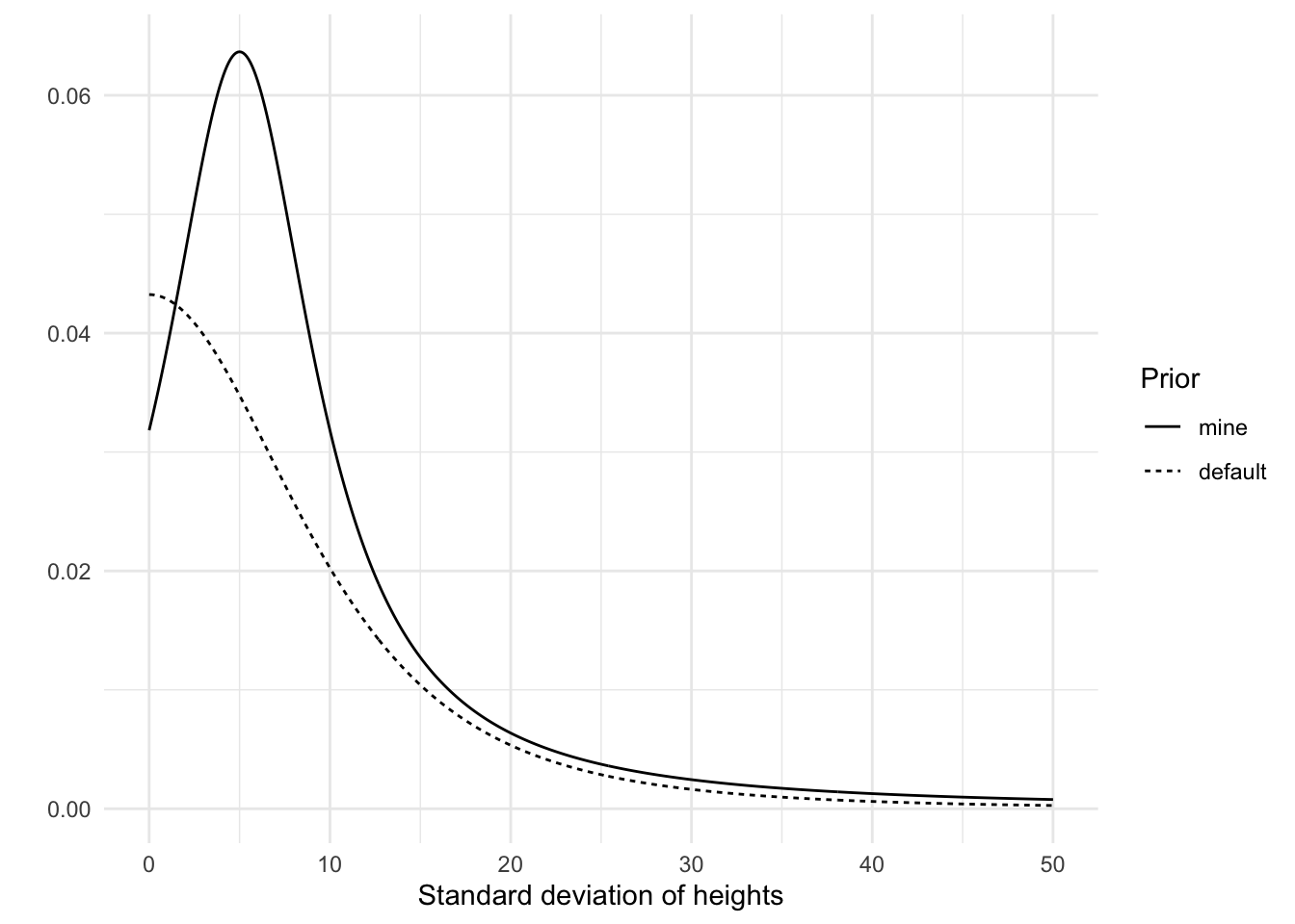
A t-distribution requires three parameters: \(\mu\), \(\sigma\), and the degrees of freedom. I set \(\mu\) to 5, \(\sigma\) to 5, and the degrees of freedom to 1. Below I plot this prior and brms’s default prior to get a better grasp of these priors.
Code
height_prior_sigma <-tibble(height_sigma =seq(from =0, to =50, by = .1),default =dstudent_t(height_sigma, df =3, mu =0, sigma =8.5),mine =dstudent_t(height_sigma, df =1, mu =5, sigma =5))height_prior_sigma <-pivot_longer( height_prior_sigma,cols =-height_sigma,names_to ="prior")ggplot( height_prior_sigma,aes(x = height_sigma, y = value, linetype =fct_rev(prior))) +geom_line() +labs(x ="Standard deviation of heights", y ="", linetype ="Prior")
Two priors for \(\sigma\)
As you can see, both distributions have longish tails, allowing for the possibility of high standard deviations. There are some notable differences between the two priors, though. My prior puts more weight on a standard deviation larger than 0, while the default prior reflects a belief in which a standard deviation of 0 is most likely. However, both priors are quite weak.
Prior predictive check
So far we have inspected each prior in isolation, but we can also use our priors to simulate heights and see if the distribution of heights makes sense. This is called a prior predictive check.
We can perform a prior predictive check using the brm() function from brms.The brm() function is the main work horse of the brms package. It enables us to run Bayesian analyses by using a common notation style familiar to those who use R. This is also one of the reasons why the brms package is so great; it’s very easy to get started with running Bayesian analyses.
The brm() function requires a model specification and the data. Optionally, but usefully, we should also specify the response distribution (a normal distribution by default) and the priors.
However, we’re not ready to actually run the model just yet. Instead, we will kinda trick brms into running an analysis, but tell it to only sample from the prior using the sample_prior argument. This will give us ‘predicted’ responses based entirely on our priors and not the data.
Additionally, we also set a seed to make the results reproducible and a file to store the results into so that if we run the analysis again, we can simply read the results from the file rather than running the analysis again. I will also set the silent argument to 2 to hide some logs that aren’t useful.
The next part is a little tricky. The goal is to obtain a large sample of predicted heights so we can visualize its distribution. By default, brms will draw 4000 draws to approximate distributions. We could use the predict() function to get these draws (e.g., predict(model_height_prior), but I prefer to use the tidybayes package because it’s a really nice package that simplifies a lot of things about working with brms models.
The tidybayes function I’ll use is add_predicted_draws(). The function takes a data frame and a model object. The function adds predictions for each row in the data frame. This is kinda tricky because we only have an intercept-only model. If you have predictors in the model you could give the function a data frame with values for each predictor that you want to obtain predicted values for. We don’t have that, so we need to give it an empty data frame. To simplify this, we’ll use a function from the modelr package called data_grid(). This function can be used to construct a data frame with predictors from the model. In this case we don’t have any predictors, but we can still specify the model. It will then create an empty data frame for us that we can add predictions to. Note that this means the data frame starts off empty but we then add draws to the data frame, creating a larger data frame.
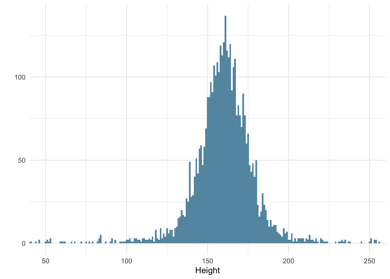
After obtaining the draws, I plot the draws using a simple histogram.
Code
heights_prior <-data_grid(.model = model_height_prior) |>add_predicted_draws(model_height_prior, value ="height")ggplot(heights_prior, aes(x = height)) +geom_histogram(binwidth =1, fill = colors[3]) +labs(x ="Height", y ="") +coord_cartesian(xlim =c(50, 250))
Prior predictive check
Our priors result in a normal distribution of heights with the bulk of the observations ranging from about 120 cm to 205 cm. That seems fairly reasonable to me, as someone who doesn’t know too much about the heights of the !Kung San.
Running the model
Now that the priors are in order we can run the model with the code below. Notice that this time I omit the sample_prior argument so we only obtain the posterior results.
Code
model_height <-brm(data = data,family = gaussian, height ~1,prior =c(prior(normal(160, 10), class ="Intercept"),prior(cauchy(5, 5), class ="sigma") ),seed =4,silent =2,file ="models/model_height.rds")
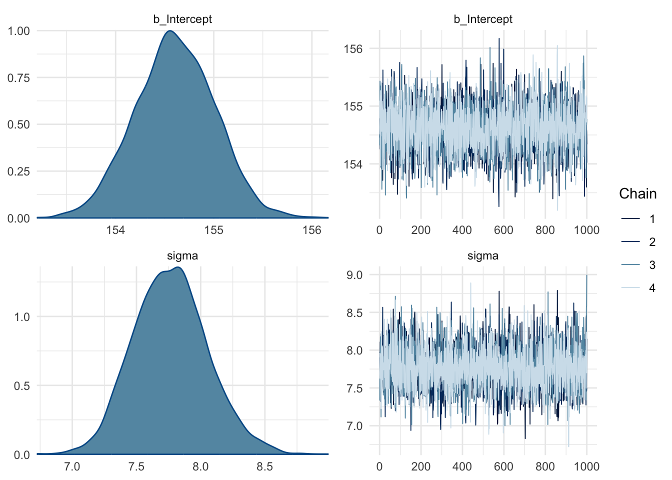
After running the model, we first check whether the chains look like caterpillars because that indicates we have samples from the entire distribution space of the posteriors.
Code
plot(model_height)
The chains look good.
We can call up the estimates and the 95% confidence intervals by printing the model object. Do note that the confidence intervals don’t have the same meaning as frequentist confidence intervals. The intervals here simply indicate what the most likely values are (given the model, priors, and data). By default, the function returns 95% intervals, meaning that 95% of the draws are between the lower and upper bounds.
Code
summary(model_height)
 Family: gaussian
  Links: mu = identity; sigma = identity
Formula: height ~ 1
   Data: data (Number of observations: 352)
  Draws: 4 chains, each with iter = 2000; warmup = 1000; thin = 1;
         total post-warmup draws = 4000

Population-Level Effects:
          Estimate Est.Error l-95% CI u-95% CI Rhat Bulk_ESS Tail_ESS
Intercept   154.61      0.41   153.83   155.39 1.00     3857     2972

Family Specific Parameters:
      Estimate Est.Error l-95% CI u-95% CI Rhat Bulk_ESS Tail_ESS
sigma     7.77      0.29     7.24     8.36 1.00     3076     2558

Draws were sampled using sample(hmc). For each parameter, Bulk_ESS
and Tail_ESS are effective sample size measures, and Rhat is the potential
scale reduction factor on split chains (at convergence, Rhat = 1).
Here we see the Intercept and sigma estimates. Apparently our posterior estimate for the Intercept is 154.61 and the estimate for \(\sigma\) is 7.77. We also see the 95% CIs, but let’s visualize these results instead.
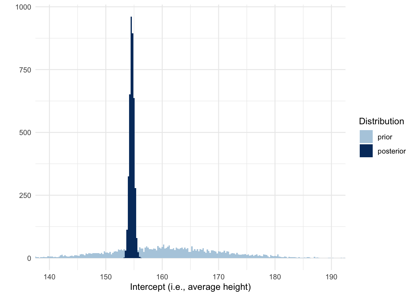
Inspecting the chains also showed us the posterior distributions of the two parameters, but let’s create our own graphs that compare both the prior and posterior distributions. We can use the spread_draws() function from tidybayes to get draws from each parameter in the model. In the code below I do that twice, once to get the draws from our previous model that sampled from the prior only and once from our new model. The result for each is a data frame and I’ll add a column to indicate whether the draw is from the prior or posterior. If you don’t know what the parameters are called, you can use the get_variables() function to get a list of the names you can extract draws from.
Here we see that the posterior distribution of average heights is much more narrow and centered around 155 cm. So not only should we switch from thinking the average is lower than 160, we can also be much more confident about the mean.
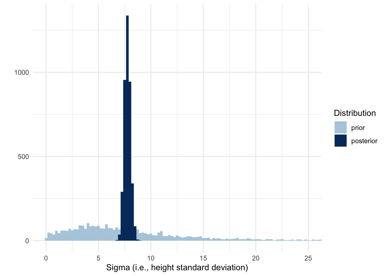
How about sigma?
Code
ggplot(draws, aes(x = sigma, fill = distribution)) +geom_histogram(binwidth =0.25, position ="identity") +labs(x ="Sigma (i.e., height standard deviation)",y ="",fill ="Distribution" ) +scale_fill_manual(values =c(colors[2], colors[5])) +coord_cartesian(xlim =c(0, 25))
Similarly, we see that the posterior for sigma is also much more narrow and around 8.
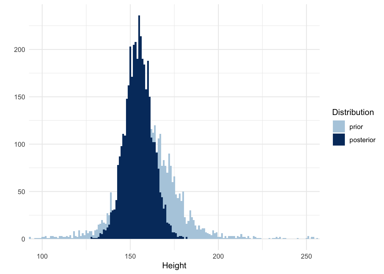
A final step is to conduct a posterior predictive check. Since we also conducted a prior predictive check we can plot both and compare how our overall beliefs about the distribution of heights should change as a function of the data. Below I create a new data frame with draws from the posterior, just like when I created the prior predictive check, and merge it with the prior data frame from before.
Code
heights_posterior <-data_grid(.model = model_height) |>add_predicted_draws(model_height, value ="height") |>mutate(distribution ="posterior")heights_prior <-mutate(heights_prior, distribution ="prior")heights <-bind_rows(heights_prior, heights_posterior) |>mutate(distribution =fct_relevel(distribution, "prior"))ggplot(heights, aes(x = height, fill = distribution)) +geom_histogram(binwidth =1, position ="identity") +labs(x ="Height", y ="", fill ="Distribution") +scale_fill_manual(values =c(colors[2], colors[5])) +coord_cartesian(xlim =c(100, 250))
Prior and posterior predictive check
This is one of my favorite plots. It shows how we started with a belief about heights and what our new belief should be, after seeing the data. That is the main goal of doing data analysis.
Summary
In this post I showed how to run an intercept-only model in brms. It consisted of the following steps:
Define the model
Use the model to figure out which priors to set
Visualize the priors and create a prior predictive check to potentially tweak the priors (using brms)
Run the model
Inspect the output, including the chains
Obtain draws of the estimates and visualize their distribution
Compare the prior predictive check to the posterior results to see how much to update based on the data
In the next post I’ll show how to add a predictor to the model.
This post was last updated on 2024-03-19.
Source Code
---title: "Bayesian tutorial: Intercept-only model"description: "The first of a series of tutorial posts on Bayesian analyses. In this post I focus on using brms to run an intercept-only regression model."date: 2023-02-01categories: - statistics - tutorial - Bayesian statistics - regressioncode-fold: truecode-tools: truetoc: truedf-print: kable---This post is the first of a series of tutorial posts on Bayesian statistics. I'm not an expert on this topic, so this tutorial is partly, if not mostly, a way for me to figure it out myself.The goal will be to go through each step of the data analysis process and make things as intuitive and clear as possible. I'll use the brms package to run the models and I will rely heavily on the book [Statistical Rethinking](https://xcelab.net/rm/statistical-rethinking/ "Statistical Rethinking website"){target="_blank"} by Richard McElreath.The basic idea behind Bayesian statistics is that we start off with prior beliefs about the parameters in the model and then update those parameter beliefs using data. That means that for all models you need to figure out what your beliefs are before running any analyses. This is very different from frequentist statistics and probably the most off-putting part of running Bayesian analyses. However, my goal is to make this relatively easy by focusing on visualizing priors and how they change as a function of the Bayesian process. I'll also try to come up with some methods to simplify the construction of priors, with the goal to have them be reasonable and non-controversial.In some cases I might not even use a prior I personally believe in. Instead I'll use a prior that represents a particular position or skepticism so that the results of the analysis can be used to change the mind of the skeptic, rather than me changing whatever I happen to believe.With this in mind, let's begin.## SetupIn the code chunk below I show some setup code to get started, starting with the packages. After loading the packages I set the default ggplot2 theme and some colors. Finally, I set several brms specific options to speed up the functions and automatically re-run models if a model has changed. If a model has not changed, the results will be read from a file instead of re-running the model.```{r}#| label: setup#| message: falselibrary(tidyverse)library(brms)library(tidybayes)library(modelr)theme_set(theme_minimal())colors <-c("#d1e1ec", "#b3cde0", "#6497b1", "#005b96", "#03396c", "#011f4b")options(mc.cores =4,brms.threads =4,brms.backend ="cmdstanr",brms.file_refit ="on_change")```## DataThe [data](Howell1.csv "Howell1 dataset"){target="_blank"} I'll use is the same data Richard McElreath uses in Chapter 4 of his amazing book Statistical Rethinking. The data consists of partial census data of the !Kung San, compiled from interviews conducted by Nancy Howell in the late 1960s. Just like in the book, I will focus only on people 18 years or older.```{r}#| label: data#| tbl-cap: Partial census data for the Dobe area !Kung San compiled by Nancy Howell in the late 1960s.#| message: falsedata <-read_csv("Howell1.csv")data <-filter(data, age >=18)head(data)```## An intercept-only modelLet's focus the first question on the heights in the data. What are the heights of the Dobe area !Kung San?The way to address this question is by constructing a model in which heights are regressed on only the intercept, i.e., an intercept-only model. You may be familiar with the R formula for this type of model: `height ~ 1`.With this formula and the data we can use brms to figure out which priors we need to set by running the `get_prior()` function. This is probably the easiest way to figure which priors you need when you're just starting out using brms.```{r}#| label: get-priorget_prior(height ~1, data = data)```The output shows us that we need to set two priors, one for the Intercept and one for sigma. brms already determined a default prior for each parameter (they are required for a Bayesian analysis), so we could immediately run an analysis if we want to but it is recommended to construct your own priors because you can often do better than the default priors.Also, using the `get_prior()` function is not the best way to think about which priors we need. Using the function will give us the answer, but it doesn't really improve our understanding of why these two priors are needed. In this case I also omitted an important specification of the heights, which is that they are normally distributed (the default in `get_prior()`). So let's instead write down the model in a different way, which explicitly specifies how we think the heights are distributed and which parameters we need to set priors on. If we think the heights are normally distributed, we define our model like this:$$heights_i ∼ Normal(\mu, \sigma)$$We explicitly note that the individual heights come from a normal distribution, which is determined by the parameters $\mu$ and $\sigma$. This then also immediately tells us that we need to set two priors, one on $\mu$ and one on $\sigma$.In our intercept-only model, the $\mu$ parameter refers to our intercept and the $\sigma$ parameter refers to, well, sigma. Sigma is not often discussed in the literature I'm familiar with, but we'll figure it out below. In fact, let's discuss each of these parameters in turn and figure out what kind of prior makes sense.## The intercept ($\mu$) priorThe prior for the intercept refers to, in this case, the *average* height of the !Kung San.brms has set the default intercept prior as a Student *t*-distribution with 3 degrees of freedom, a mean of 154.3 and a standard deviation of 8.5. That means brms starts off with a 'belief' that the average of the heights is 154.3, but with quite some uncertainty reflected in the standard deviation of 8.5 and the fact that the distribution is a Student *t*-distribution. A Student *t*-distribution has thicker tails compared to a normal distribution, meaning that numbers in the tails of the distribution are more likely compared to a normal distribution, at least when the degrees of freedom are low. At higher degrees of freedom, the *t*-distribution becomes more and more like the normal distribution. So, the thicker tails of the *t*-distributions means smaller and taller average heights are relatively more plausible.But this is the default prior. brms determines this prior by peeking at the data to create a weak prior that is easily updated by the data. We can do a bit better than the default prior, though.What do I believe the average height to be? As a Dutch person, I might think that the average height is around 175 centimeters. This is probably too tall to use as an average for the !Kung San because we're known for being quite tall. So I think the average should be lower than 175, perhaps 170. I am not very sure, though. After all, I am far from an expert on people's heights; I am only using my layman knowledge here. An average of 165 seems possible to me too. So let's describe my belief in the form of a distribution in which multiple averages are possible, to varying extents. We could use a Student *t*-distribution with small degrees of freedom if we want to allow for the possibility of being very wrong (remember, it has thicker tails, so it assigns more probability to a wider range of average heights). We're not super uncertain about people's heights, though, so let's use a normal distribution.As we saw in defining our height model, a normal distribution requires that we set two parameters: the $\mu$ and the $\sigma$. The $\mu$ we already covered (i.e., 170), so that leaves $\sigma$. Let's set this to 10 and see what happens by visualizing this prior. Below I plot both the default brms prior and our own with $\mu$ = 170 and $\sigma$ = 10.```{r}#| label: height-mu-prior#| fig-cap: Two priors for $\mu$height_prior_intercept <-tibble(height_mean =seq(from =100, to =250, by =0.1),mine =dnorm(height_mean, mean =170, sd =10),default =dstudent_t(height_mean, df =30, mu =154.3, sigma =8.5))height_prior_intercept <-pivot_longer( height_prior_intercept,cols =-height_mean,names_to ="prior")ggplot( height_prior_intercept,aes(x = height_mean, y = value, linetype =fct_rev(prior))) +geom_line() +labs(x ="Average height", y ="", linetype ="Prior") +scale_x_continuous(breaks =seq(100, 250, 20))```My prior indicates that I believe the average height to be higher than the default prior. In terms of the standard deviation, we both seem to be about equally uncertain about this average. Looking at this graph I think this prior of mine is not very plausible. Apparently I assign quite a chunk of plausibility to an average of 180 cm, or even 190 cm, which is very unlikely. An average of 160 cm is more plausible to me than an average of 180, so I should probably lower the mu, or use more of a skewed distribution. This is one of the benefits of visualizing the prior, it can make you think again about your prior so that you may improve on it. Based on the graph, I will change the mean of my prior to 160. I can probably also lower the standard deviation, but I'll leave it at 10 to show how easily the data will update this prior.## The sigma ($\sigma$) priorWhat about the sigma prior? What even is sigma? Sigma is the estimated standard deviation of the errors or, in other words, the standard deviation of the residuals of the model. In the simple case of an intercept-only model, this is identical to the standard deviation of the outcome (heights, in this case).I think setting the standard deviation of the distribution of heights (not the mean of the heights) is quite difficult. There are parts that are easy, such as the fact that the standard deviation has to be 0 or larger (it can't be negative), but exactly how large it should be, I don't know.I do know it is unlikely to be close to 0, and unlikely to be very large. That's because I know people's heights do vary, so I know the sigma can't be 0. I also know it's not super large because we don't see people who are taller than 2 meters very often. This means the peak of our prior should be somewhere above 0, with a tail to allow higher values but not too high. We can use a normal distribution for this with a mean above 0 and a particular standard deviation, and ignore everything that's smaller than 0 (brms automatically ignores negative values for $\sigma$).As I mentioned before, there is a downside of using a normal distribution, though. Normal distributions have long tails, but there is actually very little density in those tails. If we are quite uncertain about our belief about sigma, we should use a *t*-distribution, or perhaps even a cauchy distribution (actually, the cauchy distribution is a special case of the *t*-distribution; they are equivalent if the degree of freedom is 1). The lower the degrees of freedom, the more probability we assign to higher and lower values.A *t*-distribution requires three parameters: $\mu$, $\sigma$, and the degrees of freedom. I set $\mu$ to 5, $\sigma$ to 5, and the degrees of freedom to 1. Below I plot this prior and brms's default prior to get a better grasp of these priors.```{r}#| label: height-sigma-prior#| fig-cap: Two priors for $\sigma$height_prior_sigma <-tibble(height_sigma =seq(from =0, to =50, by = .1),default =dstudent_t(height_sigma, df =3, mu =0, sigma =8.5),mine =dstudent_t(height_sigma, df =1, mu =5, sigma =5))height_prior_sigma <-pivot_longer( height_prior_sigma,cols =-height_sigma,names_to ="prior")ggplot( height_prior_sigma,aes(x = height_sigma, y = value, linetype =fct_rev(prior))) +geom_line() +labs(x ="Standard deviation of heights", y ="", linetype ="Prior")```As you can see, both distributions have longish tails, allowing for the possibility of high standard deviations. There are some notable differences between the two priors, though. My prior puts more weight on a standard deviation larger than 0, while the default prior reflects a belief in which a standard deviation of 0 is most likely. However, both priors are quite weak.## Prior predictive checkSo far we have inspected each prior in isolation, but we can also use our priors to simulate heights and see if the distribution of heights makes sense. This is called a prior predictive check.We can perform a prior predictive check using the `brm()` function from brms.The `brm()` function is the main work horse of the brms package. It enables us to run Bayesian analyses by using a common notation style familiar to those who use R. This is also one of the reasons why the brms package is so great; it's very easy to get started with running Bayesian analyses.The `brm()` function requires a model specification and the data. Optionally, but usefully, we should also specify the response distribution (a normal distribution by default) and the priors.However, we're not ready to actually run the model just yet. Instead, we will kinda trick brms into running an analysis, but tell it to only sample from the prior using the `sample_prior` argument. This will give us 'predicted' responses based entirely on our priors and not the data.Additionally, we also set a seed to make the results reproducible and a file to store the results into so that if we run the analysis again, we can simply read the results from the file rather than running the analysis again. I will also set the `silent` argument to 2 to hide some logs that aren't useful.```{r}#| label: height-priormodel_height_prior <-brm( height ~1,data = data,family = gaussian,prior =c(prior(normal(160, 10), class ="Intercept", lb =0, ub =250),prior(cauchy(5, 5), class ="sigma") ),sample_prior ="only",seed =4,silent =2,file ="models/model_height_prior.rds")```The next part is a little tricky. The goal is to obtain a large sample of predicted heights so we can visualize its distribution. By default, brms will draw 4000 draws to approximate distributions. We could use the `predict()` function to get these draws (e.g., `predict(model_height_prior)`, but I prefer to use the tidybayes package because it's a really nice package that simplifies a lot of things about working with brms models.The tidybayes function I'll use is `add_predicted_draws()`. The function takes a data frame and a model object. The function adds predictions for each row in the data frame. This is kinda tricky because we only have an intercept-only model. If you have predictors in the model you could give the function a data frame with values for each predictor that you want to obtain predicted values for. We don't have that, so we need to give it an empty data frame. To simplify this, we'll use a function from the modelr package called `data_grid()`. This function can be used to construct a data frame with predictors from the model. In this case we don't have any predictors, but we can still specify the model. It will then create an empty data frame for us that we can add predictions to. Note that this means the data frame starts off empty but we then add draws to the data frame, creating a larger data frame.After obtaining the draws, I plot the draws using a simple histogram.```{r}#| label: prior-predictive#| fig-cap: Prior predictive check#| warning: falseheights_prior <-data_grid(.model = model_height_prior) |>add_predicted_draws(model_height_prior, value ="height")ggplot(heights_prior, aes(x = height)) +geom_histogram(binwidth =1, fill = colors[3]) +labs(x ="Height", y ="") +coord_cartesian(xlim =c(50, 250))```Our priors result in a normal distribution of heights with the bulk of the observations ranging from about 120 cm to 205 cm. That seems fairly reasonable to me, as someone who doesn't know too much about the heights of the !Kung San.## Running the modelNow that the priors are in order we can run the model with the code below. Notice that this time I omit the `sample_prior` argument so we only obtain the posterior results.```{r}#| label: intercept-modelmodel_height <-brm(data = data,family = gaussian, height ~1,prior =c(prior(normal(160, 10), class ="Intercept"),prior(cauchy(5, 5), class ="sigma") ),seed =4,silent =2,file ="models/model_height.rds")```After running the model, we first check whether the chains look like caterpillars because that indicates we have samples from the entire distribution space of the posteriors.```{r}#| label: chainsplot(model_height)```The chains look good.We can call up the estimates and the 95% confidence intervals by printing the model object. Do note that the confidence intervals don't have the same meaning as frequentist confidence intervals. The intervals here simply indicate what the most likely values are (given the model, priors, and data). By default, the function returns 95% intervals, meaning that 95% of the draws are between the lower and upper bounds.```{r}#| label: modelsummary(model_height)```Here we see the Intercept and sigma estimates. Apparently our posterior estimate for the Intercept is `r round(mean(as_tibble(model_height)$b_Intercept), 2)` and the estimate for $\sigma$ is `r round(mean(as_tibble(model_height)$sigma), 2)`. We also see the 95% CIs, but let's visualize these results instead.Inspecting the chains also showed us the posterior distributions of the two parameters, but let's create our own graphs that compare both the prior and posterior distributions. We can use the `spread_draws()` function from tidybayes to get draws from each parameter in the model. In the code below I do that twice, once to get the draws from our previous model that sampled from the prior only and once from our new model. The result for each is a data frame and I'll add a column to indicate whether the draw is from the prior or posterior. If you don't know what the parameters are called, you can use the `get_variables()` function to get a list of the names you can extract draws from.```{r}#| label: prior-posterior-mu#| fig-cap-: Prior vs. posterior for $\mu$#| warning: falsedraws_prior <- model_height_prior |>spread_draws(b_Intercept, sigma) |>mutate(distribution ="prior")draws_posterior <- model_height |>spread_draws(b_Intercept, sigma) |>mutate(distribution ="posterior")draws <-bind_rows(draws_prior, draws_posterior) |>mutate(distribution =fct_relevel(distribution, "prior"))ggplot(draws, aes(x = b_Intercept, fill = distribution)) +geom_histogram(binwidth =0.25, position ="identity") +labs(x ="Intercept (i.e., average height)",y ="",fill ="Distribution" ) +scale_fill_manual(values =c(colors[2], colors[5])) +coord_cartesian(xlim =c(140, 190))```Here we see that the posterior distribution of average heights is much more narrow and centered around `r round(mean(as_tibble(model_height)$b_Intercept))` cm. So not only should we switch from thinking the average is lower than 160, we can also be much more confident about the mean.How about sigma?```{r}#| label: prior-posterior-sigma#| fig-cap-: Prior vs. posterior for $\sigma$#| warning: falseggplot(draws, aes(x = sigma, fill = distribution)) +geom_histogram(binwidth =0.25, position ="identity") +labs(x ="Sigma (i.e., height standard deviation)",y ="",fill ="Distribution" ) +scale_fill_manual(values =c(colors[2], colors[5])) +coord_cartesian(xlim =c(0, 25))```Similarly, we see that the posterior for sigma is also much more narrow and around `r round(mean(as_tibble(model_height)$sigma))`.A final step is to conduct a posterior predictive check. Since we also conducted a prior predictive check we can plot both and compare how our overall beliefs about the distribution of heights should change as a function of the data. Below I create a new data frame with draws from the posterior, just like when I created the prior predictive check, and merge it with the prior data frame from before.```{r}#| label: prior-posterior-predictive-check#| fig-cap: Prior and posterior predictive check#| warning: falseheights_posterior <-data_grid(.model = model_height) |>add_predicted_draws(model_height, value ="height") |>mutate(distribution ="posterior")heights_prior <-mutate(heights_prior, distribution ="prior")heights <-bind_rows(heights_prior, heights_posterior) |>mutate(distribution =fct_relevel(distribution, "prior"))ggplot(heights, aes(x = height, fill = distribution)) +geom_histogram(binwidth =1, position ="identity") +labs(x ="Height", y ="", fill ="Distribution") +scale_fill_manual(values =c(colors[2], colors[5])) +coord_cartesian(xlim =c(100, 250))```This is one of my favorite plots. It shows how we started with a belief about heights and what our new belief should be, after seeing the data. That is the main goal of doing data analysis.## SummaryIn this post I showed how to run an intercept-only model in brms. It consisted of the following steps:1. Define the model2. Use the model to figure out which priors to set3. Visualize the priors and create a prior predictive check to potentially tweak the priors (using brms)4. Run the model5. Inspect the output, including the chains6. Obtain draws of the estimates and visualize their distribution7. Compare the prior predictive check to the posterior results to see how much to update based on the dataIn the next post I'll show how to add a predictor to the model.*This post was last updated on `r format(Sys.Date(), "%Y-%m-%d")`.*